A common use of cadCAD is to run thousands and thousands of simulations, each one with a different set of parameters and random seeds, and time and time again there is the problem of how to reliably compare the experiments, which can be very complex: they can involve a multitude of metrics as well as compositions of time series. Also, the values that arise from the models can give birth to arbitrary distributions, so that we can’t use standard analysis procedures which assume that everything is a Gaussian.
Yesterday, (and actually this post is just a summary of it) I had a discussion with @markusbkoch and @mzargham as for how reliably make sense of the estimators that we use for summarizing the distributions that arise when observing the experiments. Normally, one would use an central estimator like mean and median for aggregating the results and getting an quick view. If one goes on, he can even select an L-estimator [1]
But how much can we trust them? How reliable is the central estimator, and how can we make sense of them when needing to take a decision?
Those questions can quickly ramify into several ones, like:
- What central estimator to use?
- How to summarize the spreads and skew around the central estimator?
- How sure we are of the central estimator itself?
- How much the central estimator actually explains the data?
- What is the use case for each one?
Central estimator
The first thing is to choose the central estimator. Why would you want one anyway? Because they usually have the property of being close to the region with the highest density of points of your distribution. It is sort of an treasure map to the place where you can find most occurrences of what you are studying.
Usually, people choose either mean - because it is intuitive and converges fast, or the median, because it is robust to outliers.
The mean usually works best when your distribution is sort of a Normal one - symmetric and without additional peaks, and the median works best when the distribution is more complicated. Usually when exploring system, people tend to use the median because it is easier to become biased with the mean.
There is also a entire class of metrics that are a in-between for the mean and median. They are the L-estimators, and you can find more about them on WIkipedia [1]
Uncertainty of the data
When you have little info about the distribution itself, the best way to summarize the data is by reporting the interquartile ranges, as this captures both the variance and the skewness of the data, but still reports it in a manner that you can visualize clearly what is the applicable range of it.
Normally, you would report the median together with the 25% and 75% percentiles. So, you could express your distribution as being located at median on 12.0, with 25% / 75% percentiles on 8.0, 14.5
Uncertainty of the central estimator itself
A issue that sometimes arise with the central estimator is: how much the central estimator is uncertain by itself? When we calculate the percentile and variance of the data, we are characterizing the scale of the randomness of the process behind the data. But what about the uncertainty behind our own estimate?
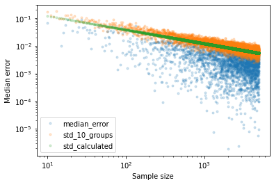
This is usually retrieved through the usage of the variance of the median, or variance of the mean if you want. In a Normal Distribution, the st. dev of the median is simply sigma_median = (pi/2)^(-1/2) * sigma / sqrt[N], where sigma is the stdev and N is the sample size. [2]
Interestingly, if you search for the st. dev for the mean, you’ll notice that it is lower by a constant factor. This means that the estimate of the mean itself is less uncertain than the median for the same amount of data. In other words: there is an trade-off between the median robustness and the speed of convergence for the mean.
That’s why you would use median for unknown distributions, and mean for simple distributions.
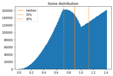
The math expression above is for a Normal distribution, but there is also the computational way of doing it, that would be to apply summarization into to the median itself. We would be looking into the median of the medians, and the variance / percentile of the medians.This usually requires characterizing / bootstrapping the distribution. Practically an simulation of the simulation. Otherwise, we would use MC runs or use grouping. If you want to, I’ve attached an notebook on this post doing this for a pathological distribution.


Uncertainty of the central estimator given the data
Now we know how uncertain is our data, how uncertain is our central estimator. How do we connect them for getting to know how uncertain is our data given our central estimator?
There are some ways for doing that, but a intuitive one is to calculate the uncertainty band, and divide it by our central estimator. The uncertainty band is the size of the variance near your central estimator, and it can be the difference of your upper and lower percentiles, or the standard deviation.
The division between the two informs how much the scale of our central estimator can be accounted by the uncertainty when looking into the data. It is sort of indicative metric really, which allows you to compare in relative fashion how much is your process being random.
When should use those uncertainty measures?
It depends where are you looking into. Analysis tasks can be sometimes divided artifiically into inference-oriented, or characterization-oriented. In the first one, you are seeking regions to where to bet your decisions, and on the second one, you are seeking to quantify how much you are sure of it.
In the first one, normally using median and the interquartile ranges are the way to go. They inform in an straightforward manner where your certainty lies.
As for the second one, the usage of the variance / estimator ratio is sometimes more useful, as it is informative of how physically meaningful are your central estimator in light of the incoming data.